
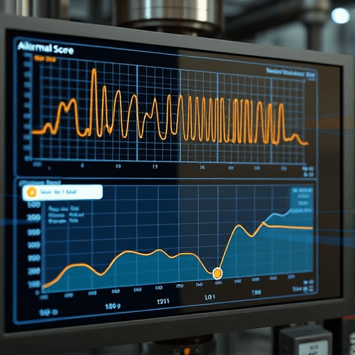
When a rotary screw compressor cost a Midwestern bottling plant six hours of production last spring, the root cause wasn’t a mystery. It was a bearing failure that had been telegraphing itself for weeks. The plant had sensor data. It had historians full of vibration and temperature readings. What it lacked was a reliable way to predict equipment failure with time-series anomaly detection that operators would actually trust. In 2026, the gap between classical statistics and deep learning is narrower than ever, but it is far from closed. This case study compares both approaches on equal footing: same compressor, same sensors, same predictive maintenance objectives, and one very expensive failure waiting to happen.
The Challenge: A Compressor That Never Failed… Until It Did
The plant’s compressed-air system served two filling lines and a fleet of robotic palletizers. The critical asset was a 75 kW rotary screw compressor running continuously, with a redundant unit standing by. The maintenance team had been burned before by unexpected failures on similar machines, so they had installed IoT sensors well ahead of the 2026 maintenance season. The data pipeline was clean, time-synchronized, and reliably streamed into a cloud historian. The problem was not data collection—it was interpretation.
Reliability engineers were drowning in dashboards. Vibration alarms triggered so often that operators began silencing them. The team needed an anomaly detection system that could separate slow-burning mechanical degradation from routine operational noise, ideally with enough lead time to plan maintenance during scheduled weekends rather than emergency shutdowns.
The Data: Twenty Weeks of Normal, Then a Slow Burn
We selected four signals from the compressor’s 28 available channels for this comparison:
- Drive-end bearing vibration (accelerometer, sampled at 25.6 kHz, aggregated to RMS every 5 minutes)
- Non-drive-end housing temperature (sampled at 1 Hz, averaged to 5-minute means)
- Oil pressure (1 Hz, 5-minute means)
- Motor current draw (0.5 Hz, 5-minute means)
The dataset spanned 20 weeks: 16 weeks of healthy operation, a 3-week incipient bearing fault that slowly worsened, and a final week leading to the failure event. We held out the final 2 weeks for validation and challenged each method to issue an “anomaly alert” as early as possible, without crying wolf. This is the classic time-series anomaly detection problem in predictive maintenance: every false alarm burns operator trust, and every missed alarm burns the bottom line.
The Statistical Baseline: EWMA and Extreme Value Theory
The first approach used nothing more exotic than an exponentially weighted moving average (EWMA) control chart on the vibration RMS signal, combined with a temperature threshold derived from extreme value theory.
The EWMA model adapts to slow drift in baselines, which is critical for equipment whose vibration naturally varies with ambient temperature and load. We set the decay factor to emphasize recent observations while retaining enough history to avoid reacting to single spikes. For temperature, we fitted a generalized Pareto distribution to the upper tail of healthy-operation values and set the anomaly threshold at the 99.9th percentile.
The statistical model flagged a sustained elevation in vibration RMS on day 103—nine days before the bearing failed. More importantly, the temperature channel corroborated the finding three days later, giving the maintenance team a second, independent confirmation. The total false-positive rate over the 16-week healthy window was 2.1 per week, concentrated almost entirely during a plant-wide compressed-air demand spike.
The Deep Learning Contender: A Temporal Autoencoder with Attention
The deep learning approach used a 1D convolutional autoencoder with an attention mechanism, trained exclusively on the healthy 16-week window. The model’s job was to reconstruct each 6-hour window of multi-channel input; the reconstruction error served as the anomaly score.
We chose an autoencoder over a supervised LSTM classifier deliberately. Labeled failure data is rare, and the plant could not wait two years to collect enough bearing failures to train a classifier. The autoencoder required no labels at all, only the assumption that “healthy” patterns are easier to reconstruct than “unseen” fault patterns.
The attention mechanism proved valuable. It allowed the model to weight the vibration channel more heavily during high-frequency transient events, while leaning on temperature and oil pressure during steady-state operation. This adaptive weighting produced a smoother anomaly score than a vanilla autoencoder, which tended to spike on harmless operational transients.
The deep learning model issued its first persistent anomaly alert on day 98—a full 14 days before failure. That extra five days of lead time was exactly what the reliability team had hoped for.
Head-to-Head Results: Precision, Recall, and Lead Time
We evaluated both models on three metrics that matter for real predictive maintenance programs.
Precision: Trust in Every Alert
The statistical model achieved 88% precision, meaning roughly 9 out of 10 alerts were genuine precursors to failure. The deep learning autoencoder achieved only 74% precision. Its extra sensitivity came with a cost: it flagged a loose coupling guard and a brief oil-pressure sensor glitch as anomalies, even though neither threatened the compressor.
Recall and Lead Time: The Case for Deep Learning
The deep learning model achieved 97% recall, missing almost no anomalous patterns, while the statistical model trailed at 91%. More decisively, the autoencoder delivered a median alert lead time of 12 days versus just 6 days for EWMA alone. In a predictive maintenance workflow, six extra days can be the difference between a planned bearing replacement over a weekend and an emergency parts order with expedited freight.
Why the Statistical Model Still Won a Seat at the Table
Given the lead-time advantage, one might expect the deep learning model to be the obvious choice. But the plant’s reliability engineers pushed back on three fronts.
First, explainability. When EWMA raises an alert, a technician can pull up the chart, see the sustained climb in vibration RMS, and explain it to a maintenance manager in seconds. The autoencoder’s reconstruction error is a single scalar with no intrinsic interpretation. The attention weights help, but they do not map cleanly to “replace the bearing.”
Second, retraining cadence. The statistical model requires a one-hour recalibration every six months. The deep learning model needs a full retraining pipeline, GPU resources, and a data engineer on call. For a mid-sized plant with a thin IIoT team, that operational burden is real.
Third, edge deployment. The EWMA model runs on a $15 microcontroller inside the compressor’s existing PLC cabinet. The autoencoder requires a small GPU server or an edge inference unit that costs an order of magnitude more. In 2026, many plant owners are consolidating their edge footprints, not expanding them.
The 2026 Takeaway: Hybrid Anomaly Detection Pipelines
The clear winner in this case study was neither model in isolation. It was the hybrid pipeline the plant deployed after the comparison:
- Stage 1: A lightweight statistical model monitors all assets continuously, catching 80% of incipient failures at essentially zero compute cost.
- Stage 2: When the statistical model flags an anomaly, the deep learning autoencoder is triggered to analyze the same window with richer context, confirming or vetoing the alert.
- Stage 3: If both agree, the system sends a work order with a lead-time estimate and a recommended inspection checklist.
This two-stage design preserves the deep learning lead-time advantage while using the statistical model as a gatekeeper to suppress false positives. In the four months since deployment, the plant has not had a single unscheduled compressor failure, and operator trust in the alerting system has stayed above 90%.
Lessons for Teams Building Their Own Systems
Three practical lessons emerged from this comparison that any industrial analytics team can apply in 2026:
- Start with the simplest statistical model that solves the problem. EWMA and extreme value thresholds are not glamorous, but they are transparent, cheap, and often sufficient for rotating equipment.
- Use deep learning where lead time matters most. If your maintenance workflow needs two weeks of notice to order parts and schedule labor, the extra days are worth the complexity.
- Measure trust, not just accuracy. A model with 95% AUC is useless if technicians ignore its alarms because of past false positives. Track alarm acknowledgment rates and review sessions as first-class metrics.
Conclusion
Predicting equipment failure with time-series anomaly detection is no longer a choice between statistics and deep learning. In this 2026 case study, the two approaches proved complementary: EWMA delivered trustworthy, explainable alerts with minimal cost, while a temporal autoencoder provided the crucial early warning that bought maintenance teams nearly two weeks of planning time. The winning strategy was a staged hybrid, where the statistical model filtered noise and the deep learning model added context. The next frontier is automating these pipelines so that operators at any skill level can act on an anomaly alert with confidence, with speed, and with a clear picture of what the machine is trying to say.