
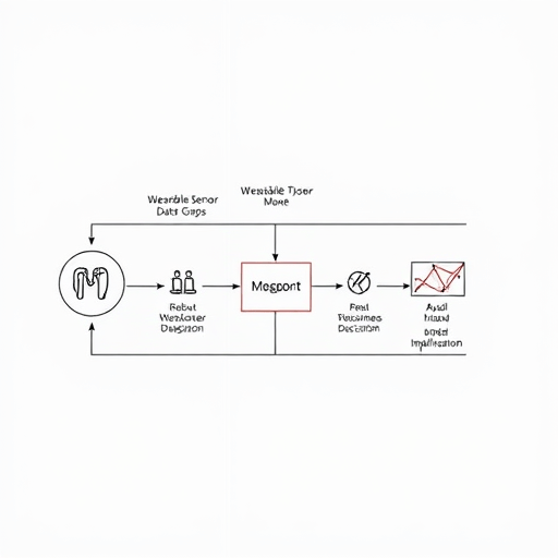
Digital biomarker validation studies hinge on continuous, high-quality sensor data—yet missingness is the rule, not the exception. Participants forget to charge wearables, remove patches during showers, or lose Bluetooth connectivity for hours. In 2026, as mobile health devices move closer to regulatory acceptance, the question is no longer whether missing data exists, but how confidently your endpoints withstand it. A sensitivity analysis framework for missing data in digital biomarker validation studies offers a systematic path to test that confidence. Rather than treating gaps as a nuisance to be filled, this framework treats them as a source of uncertainty to be explicitly modeled, stress-tested, and reported—keeping your primary endpoint robust and your conclusions defensible.
Why Missing Data Undermines Digital Biomarker Endpoints
Unlike traditional clinical measurements taken at scheduled visits, digital biomarkers produce dense, longitudinal, and often messy time series. A single day of non-wear can erase 20% of a gait feature’s data. More critically, missingness in digital datasets is rarely random. It correlates with disease severity, activity levels, sleep quality, and even socioeconomic factors—exactly the variables you are trying to measure. If ignored, sensitivity analyses become meaningless and the primary endpoint can shift from a true biological signal to an artifact of who wears the device most reliably.
The core issue is that conventional imputation methods assume missing data can be predicted from observed values. In digital biomarker studies, that assumption often fails. An older adult with Parkinson’s may remove a tremor-monitoring watch because it triggers anxiety; a patient with depression may forget to charge a smartphone because of low motivation. These missingness mechanisms are not missing at random (NMAR). A robust sensitivity analysis framework must therefore go beyond simple imputation and evaluate how different missingness assumptions alter the clinical conclusion.
Building the Framework: From Estimand to Missingness Scenarios
A modern framework aligns with the ICH E9(R1) estimand principle, adapted for sensor data. Start by explicitly defining your primary estimand—the precise clinical question your endpoint answers. For example: “mean change in nocturnal heart rate variability from baseline to week 8, regardless of wear compliance.” This definition forces you to state whether you are estimating the effect under full adherence or under real-world usage. From there, the framework proceeds through four stages: mapping missingness mechanisms, constructing plausible scenarios, applying analysis models, and aggregating results for decision-making.
Step 1: Characterize the Missingness Landscape
Before any sensitivity analysis, you must understand the patterns of data loss in your validation study. Use descriptive statistics and visualizations to classify gaps by duration, time of day, and participant characteristics. Common categories include:
- Sensor dropout – complete device failure or battery expiration, often long intervals
- Episodic non-wear – short gaps during charging, bathing, or social events
- Signal artifacts – recordings exist but are too noisy or invalid for feature extraction
- Selective non-wear – participants remove devices during specific activities or symptoms
This step is not clinical busywork—it determines which missingness assumptions your sensitivity scenarios must cover. For each category, document plausible causes and whether they relate to observed variables (e.g., time of day) or unobserved ones (e.g., sudden symptom flare). The more precise this mapping, the fewer unreasonable assumptions your analyses will need.
Step 2: Define Missingness Scenarios with Clinical Plausibility
Next, translate the missingness landscape into a set of explicit scenarios that range from optimistic to pessimistic. Each scenario encodes a different assumption about why data are missing and how those missing values might behave. For digital biomarker validation studies, four archetypes often suffice:
- Missing completely at random (MCAR) – gaps occur sporadically with no link to health state; often unrealistic but serves as a baseline
- Missing at random (MAR) – missingness is explained by observed variables like time of day, prior steps, or weekend status; implementable via multiple imputation with rich covariates
- Missing not at random (MNAR) – pattern-mixture – participants with worse symptoms are more likely to stop wearing the device; model by splitting data into compliant and non-compliant strata
- MNAR – tipping point – intensify the impact of non-wear until the primary effect loses significance; this identifies how extreme missingness must be to overturn your conclusion
The key is plausibility. In a sensitivity analysis framework, you are not looking for the model that fits best—you are testing whether your endpoint holds across a range of clinically defensible assumptions. A scenario that requires improbable changes in the missing values to flip the result increases your confidence in the endpoint.
Analytical Strategies for Each Scenario
Once scenarios are defined, choose an analysis approach that matches the missingness mechanism and the endpoint’s data structure. Do not default to a single method; the framework’s strength lies in contrasting multiple models.
Multiple Imputation with Digital Biomarker-Specific Covariates
For MCAR and MAR scenarios, multiple imputation remains a workhorse, but only if the imputation model includes the right auxiliary variables. In digital biomarker studies, these variables often include rolling means of sensor features from the previous 24 hours, day-of-week indicators, device model, and self-reported symptom diaries. The imputation model must preserve the temporal autocorrelation inherent in biosignal data; simple cross-sectional imputation will fail. Consider using predictive mean matching with lagged variables or, for larger datasets, dynamic time warping based on similar patient trajectories.
Pattern-Mixture Models for MNAR Mechanisms
Pattern-mixture models explicitly stratify participants by their missingness pattern—e.g., completers vs. non-completers—and model the endpoint separately in each stratum. These strata are then combined using weights that reflect the prevalence of each pattern. To make the model sensitivity-aware, specify clinically plausible differences between the observed and missing strata. For instance, if non-wear is linked to disease progression, you might assume that participants in the high-missingness group have a 0.5 SD worse outcome than their observed data suggest. Vary this delta across a plausible range and record the resulting effect sizes.
Tipping-Point Analysis for Regulatory-Level Robustness
Tipping-point analysis is particularly useful for validation studies intended to support a pivotal claim. For each analysis model, gradually shift the imputed values for the missing group toward the null hypothesis and observe where the primary effect loses statistical significance. The tipping point is the smallest shift that changes the study’s conclusion. If that shift is large and clinically unlikely, your endpoint is robust. If it is small—for example, requiring only a 0.1 SD difference in sensor-measured gait speed—then missingness is a serious threat to endpoint integrity, and you should redesign the study or the endpoint definition.
For digital biomarkers, tipping point analyses should be applied at the feature level, not just the final endpoint. A single sensor feature that tips easily may be driving the entire composite index. Reporting feature-level robustness prevents hidden fragility from being masked by aggregation.
Practical Implementation: Avoiding Common Pitfalls
A well-designed sensitivity analysis framework will still fail if execution is sloppy. Three pitfalls are especially prevalent in digital biomarker validation studies.
Ignoring Temporal Autocorrelation in Imputation Models
Sensor data are not exchangeable. A missing heart rate reading at 2 AM is far more similar to a reading at 1:59 AM than to one at noon. Use imputation methods that respect time series structure—ideas such as generating multiple interpolated candidates and then selecting based on dynamic time warping or state-space models. If your framework relies on standard multivariate imputation by chained equations without lagged features, it will underestimate within-person variability and overestimate precision.
Treating All Missing Data as Equivalent
A digital biomarker validation study may include dozens of sensor features. Missingness for one feature does not imply missingness for all. For example, a wrist-worn accelerometer might capture motion while the heart rate sensor fails due to poor skin contact. Your sensitivity analysis must handle feature-specific missingness, not collapse to a single binary “valid day” variable. Define missingness at the feature-session level and model joint patterns only when statistically justified.
Omitting Sensitivity Results from Regulatory Dossiers
In 2026’s regulatory environment, sponsors who report only the primary imputation analysis invite critical review. Include a dedicated appendix that details all scenario specifications, software versions, random seeds, and code. The goal is full traceability: another team should be able to reproduce your exact sensitivity analysis framework from the provided documentation. This level of transparency accelerates regulatory interactions and builds confidence among clinical collaborators.
Interpreting and Reporting Results for Decision-Making
What does a robust endpoint look like in practice? The conclusion is not a single p-value but a pattern across scenarios. When the effect size remains stable in direction and magnitude across MCAR, MAR, and mild MNAR scenarios—and only changes when the missingness assumption becomes extreme—then the endpoint is robust. Conversely, if the effect disappears or reverses in a plausible MNAR scenario, the primary endpoint is fragile, and you need to revisit either the measurement protocol, the feature selection, or the estimand itself.
Reporting this pattern is an art. Use a table or forest plot that displays the primary estimate and confidence intervals for each sensitivity scenario. Label each scenario with its clinical assumption, not just a statistical term—e.g., “assuming patients with worsening symptoms are 30% less likely to provide valid data during the final week.” This framing helps clinicians and regulators assess credibility. Additionally, compute the proportion of scenarios that support the primary conclusion; a high proportion is compelling evidence of robustness.
Conclusion
Missing data will always be a reality in digital biomarker validation studies. The question is whether your endpoints survive a structured exploration of that missingness. A sensitivity analysis framework forces intentionality: it maps how and why data disappear, defines clinically plausible alternatives, and quantifies how far you can push assumptions before your conclusions break. For research teams aiming to deliver wearable-derived endpoints that hold up under regulatory scrutiny and clinical use, such a framework is no longer optional. It is the difference between a biomarker that merely looks reliable and one that has been proven reliable under the very conditions where data are most likely to be missed.