
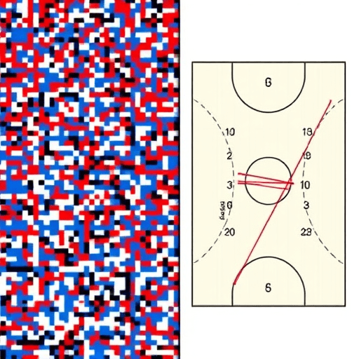
Let’s be honest: we’ve all stared at a glowing red-and-blue basketball court or soccer pitch and nodded along as the broadcaster explained that “the offense is heavily right-side dominant.” It looks scientific, decisive, and utterly modern. But if you’ve ever wondered why your favorite team’s heat map is actually useless for evaluating strategy, you’re not wrong—and you’re not alone. The truth is that the standard aggregated heat map is a statistical illusion, an artifact of overly smoothed data that strips away the most important variable in sports: context. The analytics community has largely abandoned it for a new generation of spatial tracking tools, and here is exactly what to use instead.
The Seductive But Misleading Aggregation of Spatial Data
To understand why traditional heat maps fail, you have to understand how they’re built. Most broadcast heat maps rely on Kernel Density Estimation (KDE), a statistical method that takes a scattered set of coordinate points—shots, passes, or player positions—and drapes a smooth, continuous surface over them. The problem is that smoothing inherently fabricates data. It turns a handful of isolated events into a solid “hot zone” that suggests consistency where there was only variance.
Worse, this aggregation process ignores the sequencing of events. A star point guard who logs 80% of his minutes as a pick-and-roll ball handler and 20% as an off-ball cutter will yield a heat map that shows him operating everywhere, which actually means he is effective nowhere specific. The average position of a player is a statistical fiction. Similarly, a forward who guards the opposing team’s best player in the post but zones up during blowouts will leave a map that looks like a Jackson Pollock painting—visually impressive, strategically meaningless. When you aggregate spatial data to this degree, you aren’t analyzing performance; you’re manufacturing a ghost.
Three Blind Spots Every Heat Map Misses
Beyond the math, heat maps fail fundamental eye-test scrutiny. They exist in a vacuum, devoid of the real pressures that dictate athletic success. Here are the three most damning blind spots that render them practically inert.
The Scoreboard Effect (Game State Context)
Basketball and soccer are not static environments. Teams trailing by six with four minutes left play frantic, desperate offense, attacking the rim and launching from deep. Teams leading by six compress space, bleed the shot clock, and force contested looks. A classic heat map blurs these two diametrically opposed game states into a single reddish blob, completely erasing the scoreboard effect. The result is a visualization that describes *some* basketball, but not the *specific* basketball your team actually played in the clutch.
The Ghost Defender Problem (Lack of Defensive Pressure)
A traditional shot chart only marks the location of the shooter at the moment of release. It completely ignores the defender. A catch-and-shoot three-pointer taken with five feet of clean air is charted as the exact same “hot zone” as a heavily contested step-back three taken with a hand in the shooter’s face. They are spatially identical but contextually polar opposites. By discarding the defensive geometry, the heat map rewards high-volume chuckers and punishes efficient creators who actively hunt tight coverage to draw fouls.
The Clash of Transition vs. Half-Court Execution
Nothing ruins a half-court defensive game plan like a leaky transition defense. When a team gives up easy fast-break layups, the rim becomes the reddest spot on the opponent’s heat map, even if their half-court defense is statistically elite. This conflation of pace and execution leads coaches to overreact to “rim pressure” when the actual issue is simply a lack of transition backpedaling.
What to Use Instead: Contextual Spatial Analytics
If we strip away the static heat map, what takes its place? The new wave of sports analytics leverages player-tracking cameras and machine learning to create dynamic, conditional models. These tools don’t ask *where* an event happened; they ask *why* it happened and *what was available* at that moment. Here are the three most powerful visualizations and metrics currently being adopted by forward-thinking front offices.
Possession-Segmented Shot Maps (The Filtered View)
Instead of looking at an entire game’s shot distribution, advanced analysts now use possession-segmented maps. These allow you to filter shot charts by play type (isolation, pick-and-roll, post-up, transition), by specific lineup combinations, and by game state (clutch, trailing, leading). This removes the statistical noise of the scoreboard effect and the transition clutter. A modern dashboard lets you query specifically for “what does our center shoot when guarded by a switchable wing in the fourth quarter of a one-possession game?” That’s a fragment of information a traditional heat map physically cannot provide.
Defensive Displacement and “Gravity” Maps
The future of spatial analytics isn’t about the ball—it’s about the defense. New tools utilize “Ghosting” technology to map the potential actions of a defender if an offensive player makes a certain move. These defensive displacement maps visualize the gravitational pull a star player has on all five defenders, not just the one guarding him. For example, a drive by an elite slasher causes the weak-side defender to “tag” the roller, creating a secondary pass. A heat map shows the slasher’s missed layup; a gravity map shows the open teammate he created. This shifts the focus from aggregate outcomes to process-based evaluation.
Action Probability Trees (The 2026 Evolution)
Generative AI has finally invaded the sports analytics space, and it’s producing “Action Probability Trees” or “Conditional Density Models.” Instead of mapping what happened, these models use real-time tracking data to project a branching tree of probabilities for *what will happen next* based on the current defensive alignment. Imagine a visualization that shows a 47% probability of a drive to the right, a 30% probability of a skip pass, and a 23% probability of a hand-back to the top of the key—calculated in milliseconds. This turns static analysis into a live, interactive decision-making simulator. It’s the difference between looking at a post-match weather report and looking at a live hurricane trajectory forecast.
How to Read the New Visualizations Without Losing Your Mind
If you’re a coach or a dedicated fan wanting to transition from “blob-watching” to actual insight, keep these three guidelines in mind:
- Start with percentiles, not raw totals. A player being “red hot” is useless. You need to know his expected points per possession (EPPP) against his percentile ranking for that specific play type and game state.
- Keep lineups constant. A visualization is only as good as its demographic. A map for “the team” is diluted by bench units. A map for “Starters A, B, C, D, E” is actionable gold.
- Embrace the tables of numbers. Surprisingly, the most honest spatial analysis often looks like a boring spreadsheet of expected threat (xT) values and conditional density grids before it gets translated into pretty graphics. If a visualization is trying too hard to be beautiful, it’s probably hiding a few uncomfortable truths.
Conclusion
The traditional heat map is the appendix of sports analytics—interesting to observe in a museum exhibit of early computational tools, but entirely useless for digestion or survival. It represents a bygone era where the mere existence of location data was considered a breakthrough. In 2026, the battlefield is contextual, conditional, and highly specific. To truly understand why your favorite team is winning or losing, stop staring at the red and blue blobs and start interrogating the probability trees, the defensive gravity schematics, and the segmented possession masks. That is where the actual game is won and lost.