
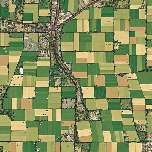
For small carbon projects, proving that soil carbon offsets are real is no longer just about earning a certificate—it is about survival in a market that has grown wary of inflated claims. The good news is that you can verify soil carbon offsets using remote sensing without the six-figure monitoring budget that once kept small developers out of the game. With open satellite archives, cloud processing, and stricter integrity standards now in place, even a small project team can build a credible and transparent verification workflow. This guide walks through that process step by step, with a focus on practical actions that reduce the risk of overcrediting.
Why Overcrediting Happens in Small Soil Carbon Projects
Soil organic carbon (SOC) is notoriously variable across even a single field. A few soil samples taken at the start and end of a crediting period can miss that variability entirely. Small projects are especially vulnerable because they often rely on sparse sampling grids, generic default values from research literature, or a handful of field plots that do not represent the full project area. Overcrediting appears when the estimated carbon gain is larger than what the soil actually sequestered. Remote sensing helps close this gap by delivering continuous, wall-to-wall coverage of the whole project area instead of extrapolating from a handful of points.
The integrity movement sweeping carbon markets has made this issue urgent. Verifiers and buyers now expect evidence that offsets are spatially explicit and statistically defensible. Satellite-based monitoring provides exactly that—if it used correctly.
Which Remote Sensing Data Actually Matter for Soil Carbon
Not every satellite image contributes equally to soil carbon verification. A cost-effective workflow should be built around three complementary data tiers.
1. Optical and Multispectral Imagery
Satellites like Sentinel-2 at 10-meter resolution and Landsat at 30-meter resolution form the backbone of soil carbon verification. Their repeated revisit time allows you to build dense time series and observe changes in soil color, surface residue, and vegetation cover—all of which correlate with soil organic matter dynamics. Indices such as NDVI and the bare soil index are useful, but they are always indirect evidence and should never be treated as direct SOC measurements.
2. Synthetic Aperture Radar
SAR sensors on satellites like Sentinel-1 and ALOS-2 penetrate cloud cover and are sensitive to surface roughness and soil moisture. These data are essential for explaining the moisture conditions that drive carbon mineralization rates. Integrating SAR alongside optical imagery can dramatically reduce uncertainty in dry seasons and tropical regions where cloud cover often obscures optical sensors.
3. Topographic and Ancillary Data
Digital elevation models from SRTM or LiDAR missions help account for slope, aspect, and drainage position—all of which influence where soil carbon accumulates or erodes. Elevation data is also useful for designing field sampling schemes that capture spatial variability rather than ignoring it.
Step-by-Step: How to Verify Soil Carbon Offsets Using Remote Sensing
Step 1 — Define the Project Boundary and Accountability Zone
Begin by mapping the precise project boundary using GPS-grade field surveys and boundary shapefiles. Remote sensing cannot fix boundary errors, and an over-reported boundary is the fastest route to overcrediting. Upload the boundary polygon into your GIS or Google Earth Engine environment and confirm it matches land tenure records.
Step 2 — Build a Baseline from Historical Imagery
Identify the longest available image archive covering your project area and select images from the same season each year. The goal is to establish a baseline trajectory of vegetation cover, bare soil exposure, and spectral variability before the project’s management changes began. For most projects, a three- to five-year historical baseline is sufficient to capture interannual climate variability.
Step 3 — Establish Calibration Plots on the Ground
Remote sensing cannot replace all field sampling—it changes how you target it. Use a stratified random sampling design based on spectral classes derived from the satellite imagery. This ensures that soil samples are collected across the full range of spectral conditions rather than clustered in accessible areas. Each calibration plot should include soil depth, bulk density, and SOC concentration measurements.
Step 4 — Model Spatial Soil Organic Carbon
Train a regression model, such as random forest or support vector regression, using the field measurements as the target and the satellite bands, spectral indices, and topographic layers as predictors. Validate the model with held-out samples and report the R-squared and root mean square error. A good model explains spatial SOC patterns while openly showing its uncertainty.
Step 5 — Track Change Over Time
Apply the calibrated model to the historical baseline images and to the monitoring images from the end of the crediting period. Subtract the two maps layer to generate a change map showing where SOC increased, decreased, or remained stable. This step recalculates the baseline internally and avoids two common errors: assuming a static baseline and ignoring natural interannual variability.
Step 6 — Calculate Conservatively Creditable Gains
Simple difference maps are not enough. To avoid overcrediting, apply a discount factor based on the confidence interval of the model prediction. Only the lower confidence bound of the estimated change should be considered creditable. This conservative approach builds verifier trust because it acknowledges uncertainty rather than hiding it.
Step 7 — Document, Audit, and Publish
Assemble a verification dossier that includes the boundary polygon, image IDs and dates, field sampling data, model code or pipeline definition, and change maps. Many registries now require this level of transparency for positive verification opinions. Publicly sharing the workflow can also serve as third-party audit evidence.
Common Pitfalls and How to Avoid Them
- Overfitting the model to a few local plots. Avoid reading too much into a handful of calibration samples. Use cross-validation and prefer simpler models when the number of field plots is small.
- Confusing vegetation greenness with soil carbon gain. A greener surface may mean more biomass, but it does not guarantee that soil carbon increased. Distinguish between aboveground biomass signals and soil reflectance signals.
- Ignoring seasonal timing. Soil moisture changes dramatically between seasons and affects reflectance. Compare images from the same calendar window each year; otherwise, the difference map may show moisture artifacts rather than carbon change.
- Omitting land-use history. Remote sensing reveals what happened, but not why. A parcel that was recently tilled or cleared requires different handling than a long-term no-till field. Document land-use history separately.
- Setting the baseline too early. If the baseline year was unusually wet or dry, the comparison will be misleading. Use an average baseline trajectory instead of a single image.
Building a Verification Workflow That Scales
Small projects often worry that remote sensing adds technical complexity. In practice, the entire workflow above can be executed in open-source tools like QGIS, Google Earth Engine, or the Python ecosystem of raster libraries. The per-project cost is primarily the time spent aligning field samples with satellite pixels, not the cost of imagery. For project developers managing multiple small parcels, a semi-automated pipeline can be reused across sites to reduce the marginal cost of verification to near zero.
Another advantage of this approach is its auditability. Unlike manual photo interpretation, spectral index thresholds can be revisited. The model’s assumptions can be tested by a verifier without needing access to the original analyst’s judgment. That transparency is exactly what the 2026 carbon market needs as regulators and buyers push for greater certainty in soil carbon accounting.
Finally, remember that remote sensing does not replace good agronomy. Management interventions like cover cropping, no-till, and compost application must be documented as well. The most defensible projects combine remote sensing verification with rigorous practice records.
Conclusion
Verifying soil carbon offsets using remote sensing is now a realistic pathway for small projects that want to avoid overcrediting and build long-term market credibility. By combining free satellite imagery, a modest number of strategically located field samples, and transparent statistical modeling, a small project can produce spatially explicit carbon estimates that withstand scrutiny. The key is to treat remote sensing not as a magical replacement for soil sampling, but as a powerful tool for scaling field truths across an entire landscape. Small projects that adopt this approach early will be ready for the higher integrity standards ahead—and far less likely to see their credits challenged.