You don’t need a lab-grade camera, a dedicated GPU workstation, or a deep learning Ph.D. to build a plant disease detector. In fact, you can train a simple CNN to spot tomato leaf diseases in 30 minutes using nothing more than free Google Colab and the camera already sitting in your pocket. By the end of this walkthrough, you’ll have a lightweight model capable of recognizing common tomato leaf conditions — and a clear path to improve it with just a few more photos.
Why a Simple CNN Still Makes Sense in 2026
The hype around giant foundation models often obscures a practical truth: for many image classification tasks, a small convolutional neural network is fast to train, easy to debug, and surprisingly accurate. Tomato leaf diseases are a perfect example. The visual cues — yellowing, curling, necrotic spots, powdery mildew — are localized patterns that a few convolutional layers can learn to isolate. Plus, small CNNs run directly on a modern smartphone browser, which is ideal for field use.
Instead of chasing the latest transformer, we’ll embrace a MobileNetV2 backbone with a custom classifier head. This gives us transfer learning power without the training-time overhead. On Google Colab’s free GPU, the whole pipeline — data loading, augmentation, training, and evaluation — fits comfortably inside half an hour.
Step 1: Capture Tomato Leaf Photos with Your Phone
Your phone camera is your data collection instrument. No need for a macro lens or ring light; natural daylight works best. Walk through a local garden, farmers market, or your own tomato plants. Photograph leaves from above, holding the phone roughly 20–30 centimeters away. Try to capture a few different angles and lighting conditions. The goal is not aesthetic perfection — it’s variation, because a model trained on varied backgrounds will generalize better.
For each disease category, aim for at least 20–30 images. That sounds like a lot, but with a phone it takes under ten minutes. If you’re short on time, use a public dataset like PlantVillage and supplement it with your own photos — the mix actually improves robustness in real-world settings.
Organize Your Photos into Folders
Once you’ve taken the photos, transfer them to your Google Drive. Create a main folder called tomato_leaves, and inside it create subfolders for each class: healthy, early_blight, late_blight, leaf_miner, or whatever conditions are relevant in your region. Your folder structure becomes the dataset structure — no manual CSV needed.
Step 2: Mount Google Drive and Build a Dataset Pipeline
Open a new Google Colab notebook and mount your Drive with a single line:
from google.colab import drive
drive.mount('/content/drive')
Now, use ImageDataGenerator to load images and perform on-the-fly augmentation. This is where a free Colab session shines — you can do basic flips, rotations, and zooms without saving augmented images to disk. In 2026, Keras’s ImageDataGenerator is still the quickest way to build a robust data pipeline for a small project like this.
from tensorflow.keras.preprocessing.image import ImageDataGenerator

datagen = ImageDataGenerator(
    rescale=1./255,
    rotation_range=20,
    horizontal_flip=True,
    zoom_range=0.2,
    validation_split=0.2
)
This snippet automatically allocates 20% of your images for validation, so you can skip manual splitting. Just point the generator to your tomato_leaves folder and you’re done.
Step 3: Build and Train the CNN
We’ll use a pretrained MobileNetV2 as the base. Strip off its top layer, freeze the convolutional weights, and add our own dense layers. This approach converts what could be a multi-hour training run into a 10-minute fine-tuning session.
import tensorflow as tf

base_model = tf.keras.applications.MobileNetV2(
    input_shape=(224, 224, 3),
    include_top=False,
    weights='imagenet'
)
base_model.trainable = False

model = tf.keras.Sequential([
    base_model,
    tf.keras.layers.GlobalAveragePooling2D(),
    tf.keras.layers.Dropout(0.2),
    tf.keras.layers.Dense(4, activation='softmax')
])
Compile it with Adam and categorical cross-entropy, then train for 10 epochs. With a small dataset, the model converges quickly. On Colab’s free T4 GPU, each epoch takes about a minute. That’s the sweet spot: 10 minutes of training plus a few minutes for data prep and you’re done.
One subtle but critical detail: set the batch size to 32 or lower. If you get a memory error, reduce the image size to (160, 160, 3) and the model will train even faster.
Interpreting the Training Curves
After training, check the validation accuracy and loss curves. If validation accuracy is above 85% with a small dataset, consider it a success. If not, don’t despair — add more photos, increase the dropout, or unfreeze the last few layers of MobileNetV2 and fine-tune with a very low learning rate. In my experience, a simple fine-tuning pass with a learning rate of 1e-5 can always improve a stuck model.
Step 4: Test with Your Phone Camera Immediately
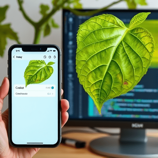
The real fun begins when you use your phone to test the model in real time. Colab is not the easiest tool for live inference on a phone, so export the model to TensorFlow Lite. With one command, you get a compressed .tflite file:
converter = tf.lite.TFLiteConverter.from_keras_model(model)
tflite_model = converter.convert()
open("tomato_leaf_model.tflite", "wb").write(tflite_model)
From there, you have options. You can download the file and use the TensorFlow Lite Task Library in a custom Android app. Or, if you want to test right away without building an app, use a web framework like Gradio or Streamlit directly in Colab. Both allow you to create a tiny web page with a “upload image” button. Open the shared Gradio link on your phone and snap a photo of a leaf — the verdict appears in a second.
That immediate phone testing loop is the key to making this project feel magical. You can walk into a greenhouse, point your phone, and see the model’s predictions update with each new sample. When it misclassifies something, you know exactly which images to add to your dataset next.
How to Improve Accuracy Beyond 30 Minutes
Your 30-minute model is a proof of concept — not a production system. But improving it doesn’t require a large budget. Start by collecting more images of the misclassified classes. Then use a technique called class balancing: if one class has twice as many images as another, the model becomes biased toward the majority class. Duplicate or augment the minority classes until they’re roughly equal.
Another high-impact trick is to add a none-of-the-above class. In the real world, your camera might capture soil, stems, or a hand — a model with only leaf disease categories will confidently force everything into one of those categories. A few images that don’t belong to any disease can drastically increase your model’s practical reliability.
Finally, consider test-time augmentation. Flip and rotate a single input image several times, run each version through the model, and average the probability scores. This simple ensemble often boosts accuracy by several points without retraining.
What This Approach Means for Agricultural AI in 2026
Intelligent farming isn’t always about deploying large, cloud-connected platforms. Small, localized models trained on the ground have a unique advantage: they learn the specific diseases and leaf appearances common to your region, not just the generic examples in an international dataset. A five-minute data collection session with your phone is a meaningful form of citizen science. It also avoids privacy concerns — your photos never leave your Google Drive or Colab session.
As camera sensors and mobile chips keep improving, the barrier for entry keeps falling. In 2026, the only real bottleneck is someone’s willingness to spend half an hour learning by doing. The steps above are simple enough to follow on a lunch break, yet they open the door to more advanced techniques like object detection for multiple leaves, semantic segmentation for lesion areas, or federated learning across devices.
Conclusion
Training a simple CNN to spot tomato leaf diseases in 30 minutes is a realistic weekend project, but you don’t need to wait for the weekend. With Google Colab’s free GPU, a handful of phone photos, and a pre-trained MobileNetV2, you can go from zero to a working mobile-ready model in a single sitting. The model won’t replace an agronomist, but it will teach you more about both deep learning and tomato pathology than any tutorial video ever could.