
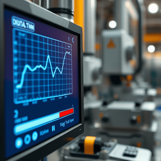
Keeping a digital twin perfectly in lockstep with the physical factory floor has always been the holy grail of industrial digitalization. Yet as operations embrace more connected assets, the gap between modeled behavior and actual sensor readings becomes the critical bottleneck. This article walks through a pragmatic, step-by-step approach to syncing digital twin models with live factory data, using IoT sensor time-series as the calibration backbone. Instead of treating calibration as a one-time setup, we’ll focus on establishing a continuous, automated rhythm—one that fits the modern, data-rich factory environment of 2026.
The Shift from Static Twins to Living Models
Most digital twin projects start with a burst of enthusiasm: a detailed CAD model, a handful of historical IoT logs, and a simulation that matches past performance to the decimal point. But the moment production ramps up or ambient conditions change, the twin drifts. The sensors keep streaming second-by-second values, but your model slowly becomes a beautiful, static artifact. In 2026, the expectation is no longer a one-time snapshot of accuracy—it’s a twin that breathes with the factory.
This requires moving from a “build and validate” mindset to a “continuously calibrate” mindset. The good news? IoT time-series data is precisely the signal you need to keep the model alive. The challenge is knowing how to feed that signal into the model in a way that doesn’t introduce noise, overfitting, or brittle recalibration loops. The following steps give you a structured path—designed to be practical, not theoretical.
Step 1: Align Your Telemetry Schema with the Twin’s Semantic Layer
Before any math happens, you need a shared language. If your sensor IDs, units, and data types don’t match your digital twin’s internal model parameters, synchronization is impossible. Start by mapping every live IoT telemetry stream to the corresponding digital twin input. For example, a vibration sensor on a motor might feed the imbalance force parameter, while a current transducer maps to torque demand. This mapping is often called a semantic layer.
Define a Canonical Time-Series Format
- Use ISO 8601 timestamps with timezone offsets—no exceptions.
- Store all values as doubles, but keep the original unit in metadata.
- Maintain a consistent sampling interval (e.g., 1 second) or store timestamps per sample and resample internally.
- Add a sensor health field to flag stuck values or out-of-range readings.
Your digital twin platform should expose a configuration file or API that lists every input parameter and its accepted unit. Compare that list with your IoT data stream’s metadata. The alignment here saves hours of debugging later.
Step 2: Curate and Clean Raw IoT Time-Series for Calibration
Raw sensor data is messy. Disconnected gateways, brief power outages, and electromagnetic spikes create gaps and outliers. If you feed that directly into a calibration algorithm, your digital twin will chase ghosts. Time-series cleaning is not about deleting data—it’s about making the data usable for parameter estimation.
Practical Cleaning Sequence
- Remove samples with invalid sensor status flags (e.g., device heartbeat lost).
- Apply a spike filter (e.g., a rolling median with a 3-window threshold) to eliminate transient surges.
- Interpolate missing data only if the gap is smaller than 10% of the calibration window length.
- Normalize the data to the same time grid as your twin’s simulation step.
One habit worth adopting: keep a separate “raw” store and a “clean” store. This allows you to trace every calibration input back to its original signal and audit the cleaning logic.
Step 3: Define Calibration Triggers and Drift Thresholds
You don’t need to recalibrate every second. The key is knowing when the twin’s output has deviated enough to warrant intervention. Instead of running a full parameter optimization on every batch, define drift thresholds based on the criticality of each parameter. For instance, temperature estimates might tolerate a 2°C offset, while pressure setpoints may require a 0.5% match.
Build a Drift Detection Rule
Use a sliding window of the last N prediction-vs-actual pairs. Compute the mean absolute error (MAE) or root mean square error (RMSE) over that window. If the error exceeds your threshold for three consecutive windows, flag the digital twin as “out of sync.” This is the trigger for the calibration routine. For automated environments, make the trigger an event that writes a recalibration ticket or invokes a serverless function.
Step 4: Run the Calibration Loop with a Sliding Window
Now we get to the core: actually updating the model parameters. The goal is to estimate the parameters that minimize the error between the simulated outputs and the live sensor measurements. A common and effective method is to use a sliding window of time-series data—typically 24 to 72 hours of operational history. This window should be short enough to reflect current conditions but long enough to cover a representative range of operational states.
Parameter Estimation Techniques
- Gradient-based optimization: Fast for smooth loss surfaces, but sensitive to initialization.
- Particle swarm or genetic algorithms: More robust to local minima, but slower to converge.
- Bayesian calibration: Produces a posterior distribution of parameters—great for uncertainty-aware twins.
During the calibration step, freeze the model’s equations and only adjust the coefficients that are physically plausible (e.g., heat transfer coefficient, damping factor, friction constant). Do not touch structural parameters like geometry or material type unless your validation step explicitly shows an error pattern that cannot be corrected otherwise. After the optimization run, compare the calibrated twin’s output against a separate validation dataset—not the same window used for fitting.
Step 5: Validate with a Holdout Set and Live Shadow Mode
Calibration without validation is just curve fitting. Always hold out a slice of recent time-series data—say the last 12 hours—that the optimization algorithm never sees. After updating the model parameters, run the twin against that holdout set and measure its performance. If the error is still above the threshold, something more fundamental might be wrong with your model structure, not just the coefficients.
For extra confidence, run the updated twin in shadow mode: the twin predicts along with the live sensor feed, but nothing is written back to the operational system. During shadow mode, monitor the error trend for several hours or days. Only promote a recalibrated twin to active status when it can maintain low error on unseen, live data.
Step 6: Automate Recalibration Through a Feedback Loop
Manual recalibration is acceptable for a pilot, but a synchronized digital twin in production needs automation. Build a feedback loop that connects the drift detector, the optimizer, and the promotion pipeline. A simple architecture might look like this:
- An IoT gateway pushes time-series data to a stream processing engine.
- The engine calculates rolling error metrics and emits drift events.
- A workflow orchestrator triggers the calibration job with the current sliding window.
- The job saves the new parameter set and runs validation tests.
- If validation passes, the new parameter set is deployed to the twin runtime and logged.
This loop should run on a cadence that matches your factory’s dynamics—perhaps hourly, every shift, or daily. In some edge environments, the entire loop can run locally on a gateway or industrial PC, reducing latency and avoiding cloud dependency.
Handling Non-Stationary Behavior and Concept Drift
Factory processes are rarely stationary. Tool wear, raw material variability, and changing ambient conditions mean the “right” parameters evolve over time. Your calibration method must be able to adapt to slow drift and sudden changes. One technique is to weight recent samples more heavily in the loss function. Another is to maintain an ensemble of twin configurations and switch among them based on the current operating mode. For example, a machine tool might have different calibration profiles for roughing and finishing passes. Let the time-series characteristic—like spindle load pattern—select the appropriate profile.
Conclusion
Syncing digital twin models with live factory data is not a one-time project; it is a discipline. By aligning telemetry schemas, cleaning time-series streams, defining drift thresholds, and running a sliding-window calibration loop with proper validation, you can keep the digital twin honest and operationally relevant. As factory data grows richer and more real-time, the factories that master this synchronization will be the ones that can trust their virtual counterparts for decisions—not just for dashboards. Start with a single line or asset, prove the loop, and then scale it across the floor.