When a payment API starts adding 400 ms to its p99 right before Black Friday, the trace that proves why is usually the one your sampler decided not to keep. Engineers running distributed systems on Kubernetes face a recurring bind: keep every trace and your observability bill explodes, sample aggressively and you lose the rare, expensive failures that actually matter. The fix is not a single sampling strategy but an adaptive OpenTelemetry sampling pipeline that toggles between head-based and tail-based collection on the fly, weighted by service-specific SLO budgets. This guide walks through a working pattern for doing exactly that on clusters running in 2026, where trace volumes have quietly become a top-three cost driver for many platform teams.
Why static sampling fails at scale
Most teams start with a fixed head-based sampler on the OpenTelemetry Collector: keep 5% of traces, drop the rest, move on. It is cheap and predictable. It is also blind. A head-based decision is made the instant the root span is created, before latency, error status, or downstream behavior is known. That means the exact traces you most want, the slow checkout, the timed-out webhook, the cascading retry storm, are statistically as likely to be discarded as a healthy 30 ms request.
Tail-based sampling solves the visibility problem but introduces a new one: the collector must buffer every span in memory or on disk until the trace completes, then decide whether to keep it. At a few hundred requests per second that is fine. At tens of thousands, buffer pressure alone can become its own outage. The result is that teams either over-sample and bleed budget, or under-sample and miss incidents.
The insight behind adaptive sampling is that you rarely want one mode all the time. During a normal Tuesday morning you do not need every trace. During a p99 excursion on a revenue-critical service, you do.
The shape of an adaptive pipeline
An adaptive sampler treats the cluster as a dynamic system and reacts to its state. Three building blocks make it work:
- An SLO budget map that declares, per service, how much error budget remains for the current burn period. The classic Google SRE formulation works well here: a 30-day target of 99.9% availability gives you roughly 43 minutes of allowed downtime, tracked hour by hour.
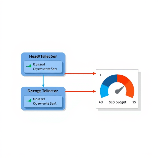
- A head-based OTel Collector deployed as a DaemonSet on each node, responsible for the cheap, local decision: keep this trace or buffer it for review.
- A tail-based OTel Collector running as a Deployment with persistent volume claims, where final keep-or-drop decisions are made once the trace closes and SLO state is known.
The head collectors apply a probabilistic baseline, say 2%, plus a small always-on population for known-noisy endpoints. They forward everything, including dropped traces, by writing to a local ring buffer with a configurable retention window. The tail collector drains that buffer, evaluates each trace against the live SLO budget for the originating service, and decides.
Encoding SLO budgets as sampling weights
The core of the technique is converting remaining error budget into a sampling probability. A simple model that works in practice:
- If a service has more than 50% of its monthly error budget remaining, sample at the baseline rate (2%).
- If it has between 20% and 50% remaining, raise the rate to 10%, capturing more latency outliers before they erode the budget.
- If it has under 20% remaining, switch to 100% capture for that service until the burn rate normalizes.
This produces a smooth, automatic escalation. Healthy services stay cheap. Services approaching their SLO limit become expensive, deliberately, because the marginal cost of an extra gigabyte of traces is far less than the cost of missing the root cause of a regression.
The budget state itself lives in a small Redis or etcd-backed key that the tail collector reads on each evaluation. The head collectors periodically pull a compressed version of the map through a Collector extension so they can adjust their forwarding probabilities without round-tripping on every span.
Building the Kubernetes deployment
Three manifests matter most. First, the head Collector as a DaemonSet with resource requests tuned conservatively. Memory is the constraint: a 30-second ring buffer at 5,000 spans per second per node needs roughly 2 to 4 GB depending on span cardinality. Set limit_memory generously and use the OTel Collector’s own memory limiter processor to shed load gracefully.
Second, the tail Collector as a StatefulSet with a PersistentVolumeClaim per replica sized for at least 10 minutes of worst-case trace volume. Horizontal Pod Autoscaler reacts to buffer depth, not CPU, since the workload is I/O bound.
Third, a ConfigMap that holds the SLO budget map and a small CronJob that recomputes burn rates every five minutes from Prometheus and rewrites the ConfigMap. Most teams already have the multi-window multi-burn-rate alerts from the Google SRE workbook; this job simply reads the same counters and publishes a sampling-friendly derivative.
Avoiding the common failure modes
Three pitfalls deserve attention. The first is head-of-line blocking when the tail collector falls behind. Set a hard deadline on trace assembly and ship whatever is complete at that point, even if some spans are missing. Partial traces are dramatically more useful than no traces.
The second is cardinality explosion in the sampling decision itself. If your SLO key includes raw URLs or user IDs, you will regret it fast. Hash service identity and route template, nothing finer.
The third is tail latency from your own pipeline. Adaptive sampling helps your application; it should not become the next incident. Run the tail collector on a dedicated node pool with guaranteed QoS, and isolate its network path from production traffic. Add a synthetic trace generator that injects a known-bad span every minute and assert the pipeline keeps it within ten seconds end to end.
What changes operationally
Once the adaptive loop is live, the on-call experience shifts in a useful way. During a quiet week the bill looks like the old 5% baseline. During an incident, trace volume spikes for exactly the services that matter and stays flat for the rest. Postmortems stop containing sentences like “we cannot reproduce because the trace was sampled out.” Platform engineers stop negotiating with finance about whether observability is a luxury.
Cost savings typically land between 40% and 70% versus naive always-on tail sampling, while error-detection latency for SLO-relevant services drops to near real time. The trade is real complexity: two collectors, a budget service, and a config pipeline. For any organization past a handful of services and a few thousand requests per second, that complexity pays for itself inside one quarter.
The biggest lesson from teams that have run this pattern for a while is that sampling is not a static configuration choice but an extension of your reliability posture. Treat your SLOs as live inputs to your observability pipeline, and your traces start telling the truth at exactly the moments that truth matters most.