AI‑Driven Crop Yield Forecasting for Home‑Grown Hydroponic Systems

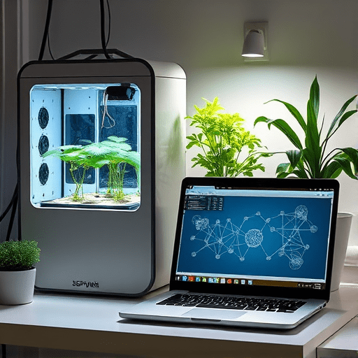
Growing food at home has never been easier—especially with hydroponic systems that deliver precise nutrient delivery, controlled lighting, and efficient water usage. But even the most meticulous growers face the question: how much will my lettuce or tomato yield tomorrow? The answer lies in data: real‑time sensor readings and local weather forecasts. By building a lightweight neural‑network model, you can transform raw data into actionable yield predictions that help you plan harvests, optimize resources, and increase profitability. In this step‑by‑step guide we’ll walk through the entire pipeline—from data collection and preprocessing to model training, evaluation, and deployment—so you can start forecasting daily yields in your own home‑grown hydroponic garden in 2026.

1. Gather and Prepare the Data

The foundation of any AI model is high‑quality data. For a hydroponic system, your data sources typically include:

• Sensor Data: pH, EC (electrical conductivity), nutrient concentration, water temperature, air temperature, relative humidity, CO₂ level, and LED light intensity.
• Weather Feed: Local temperature, humidity, UV index, precipitation probability, wind speed, and daylight hours.
• Growth Log: Daily records of plant height, leaf count, and any manual interventions (e.g., pruning, nutrient adjustments).
• Yield Records: Actual harvest weight per day or per plant.

Collect data at a consistent frequency—ideally every 15 minutes for sensors and hourly for weather. Store the data in a CSV or a lightweight database like SQLite. Ensure timestamps are synchronized to avoid misaligned features.

Next, clean the data:

• Remove outliers using z‑score thresholds (values > 3 σ).
• Fill missing values with interpolation or forward‑fill methods.
• Normalize continuous features to a 0–1 range using Min‑Max scaling.
• Create lag features (e.g., sensor reading 3 hours ago) to capture temporal dependencies.

Finally, split the data into training, validation, and test sets (e.g., 70/15/15). Keep the test set strictly for final evaluation to avoid data leakage.

2. Feature Engineering for Yield Prediction

While raw sensor data is valuable, carefully engineered features can boost model performance:

• Time‑of‑Day Indicator: Binary features for morning, afternoon, evening, and night to capture light intensity changes.
• Weather Trend: Rolling averages of temperature and humidity over the past 12 hours.
• Growth Rate: Difference between current and previous height measurements.
• Nutrient Uptake Estimate: Integrate EC and pH to approximate nutrient availability.
• Light Saturation Index: Ratio of current LED intensity to the system’s maximum output.

Encode categorical variables (e.g., plant variety) using one‑hot encoding. Drop any features with near‑zero variance to reduce dimensionality.

3. Choose the Neural‑Network Architecture

For daily yield forecasting, a Temporal Convolutional Network (TCN) or a shallow Long Short‑Term Memory (LSTM) network is effective. Both capture temporal dependencies without excessive computational cost, making them suitable for a Raspberry Pi‑based deployment.

Below is a simple LSTM architecture implemented in TensorFlow/Keras:

import tensorflow as tf
from tensorflow.keras import layers, models

def build_model(input_shape):
    model = models.Sequential()
    model.add(layers.Input(shape=input_shape))
    model.add(layers.LSTM(64, return_sequences=False))
    model.add(layers.Dense(32, activation='relu'))
    model.add(layers.Dense(1, activation='linear'))  # Predict yield in grams
    model.compile(optimizer='adam', loss='mse', metrics=['mae'])
    return model

Key hyperparameters to tune:

• Number of LSTM units (32–128)
• Learning rate (1e-3 to 1e-4)
• Batch size (32–128)
• Number of epochs (30–100, with early stopping)

Use EarlyStopping on validation loss to prevent overfitting.

4. Train the Model

Prepare the data for the LSTM by reshaping it to (samples, timesteps, features). For example, if you use a 6‑hour window with 15‑minute intervals, you’ll have 24 timesteps per sample.

import numpy as np

def create_sequences(df, seq_length=24):
    X, y = [], []
    for i in range(len(df) - seq_length):
        X.append(df.iloc[i:i+seq_length].values)
        y.append(df.iloc[i+seq_length]['yield'])
    return np.array(X), np.array(y)

X_train, y_train = create_sequences(train_df)
X_val, y_val = create_sequences(val_df)

Fit the model:

model = build_model(input_shape=(X_train.shape[1], X_train.shape[2]))
history = model.fit(
    X_train, y_train,
    validation_data=(X_val, y_val),
    epochs=50,
    batch_size=64,
    callbacks=[tf.keras.callbacks.EarlyStopping(patience=5, restore_best_weights=True)]
)

After training, evaluate on the test set:

test_loss, test_mae = model.evaluate(X_test, y_test)
print(f"Test MAE: {test_mae:.2f} g")

5. Interpret and Validate the Model

Use SHAP or LIME to interpret feature importance. For instance, SHAP may reveal that recent temperature and CO₂ levels are the strongest predictors of yield. Plot the predicted vs. actual yields to visually assess model performance.

Validate on a held‑out period (e.g., the last month) to ensure the model generalizes across different growth cycles and weather patterns.

6. Deploy on the Edge

For real‑time forecasting, deploy the model on a low‑power device like a Raspberry Pi 4 or an Arduino with TensorFlow Lite support.

• Convert to TensorFlow Lite: tf.lite.TFLiteConverter.from_keras_model(model)
• Bundle with sensor API: Write a Python script that reads sensor data every 15 minutes, feeds it to the TFLite model, and outputs a daily yield prediction.
• Store predictions: Append to a local CSV or send via MQTT to a cloud dashboard.

Example inference loop:

import time
import numpy as np
import tflite_runtime.interpreter as tflite

interpreter = tflite.Interpreter(model_path="model.tflite")
interpreter.allocate_tensors()

while True:
    sensor_data = read_sensors()  # custom function
    weather_data = fetch_weather()  # API call
    input_array = preprocess(sensor_data, weather_data)
    input_data = np.array([input_array], dtype=np.float32)
    
    interpreter.set_tensor(interpreter.get_input_details()[0]['index'], input_data)
    interpreter.invoke()
    prediction = interpreter.get_tensor(interpreter.get_output_details()[0]['index'])[0]
    log_prediction(prediction)
    time.sleep(900)  # 15 minutes

7. Continuous Learning and Model Updating

Plant growth dynamics can shift due to new seed batches, changing environmental conditions, or system modifications. Implement a feedback loop that retrains the model monthly using the latest yield records.

• Automate data ingestion and preprocessing with cron jobs.
• Monitor performance metrics; if MAE rises above a threshold (e.g., 10 % higher than baseline), trigger a retrain.
• Version‑control models using a lightweight model registry (e.g., MLflow or a simple Git repository).

By keeping the model up‑to‑date, you maintain high forecast accuracy throughout the growing season.

8. Expanding Beyond Yield: Predicting Quality and Nutrient Deficiencies

Once you’ve mastered yield forecasting, extend the model to predict:

• Leaf chlorophyll index for nutritional content.
• Time to reach market size for scheduling harvests.
• Early warning signals for nutrient imbalances or pest infestations.

These additional predictions further optimize resource use and product quality, turning a simple hydroponic setup into a data‑driven production system.

9. Common Pitfalls and How to Avoid Them

• Data Drift: Regularly compare sensor statistics to training data; adjust preprocessing if distributions shift.
• Overfitting: Keep the network shallow and use dropout layers if necessary.
• Hardware Limitations: Quantize the model to 8‑bit integers for faster inference on edge devices.
• Missing Weather Data: Cache weather forecasts locally to prevent API outages from breaking predictions.

10. Resources for Further Exploration

Below are links to open‑source projects and libraries that can help you build and refine your system:

• AirVisual API for air quality data
• Temporal Convolutional Networks in Keras
• Keras documentation
• TensorFlow Lite for edge deployment

These resources provide code examples, tutorials, and community support to deepen your understanding and accelerate development.

By following this guide, you’ll turn raw sensor data and weather feeds into actionable, daily yield predictions that empower your hydroponic hobby or small‑scale commercial operation. Embrace the data, iterate quickly, and watch your garden thrive with precision AI.